Lab 1 · Chance, repetition, and fair tests

Level: Levels 1–2 · Prerequisites: L1-02 (probability model), L1-03 (repeat and record), L1-05 (assign a fair comparison)

What you’ll learn:

A probability belongs to a model. A relative frequency is a measurement, and it can differ from the model.
Many independent trials usually bring the frequency close to the model probability. This is the law of large numbers. You will also see how big the typical gap is.
A 95 % band around the probability is about one fixed number of trials. It says nothing about a whole run.
A coin flip that assigns the treatment balances a hidden trait on average. Letting people choose does not.

import sys, pathlib, subprocess
here = pathlib.Path.cwd()
root = next((p for p in [here, *here.parents] if (p / "qcai").is_dir()), None)
if root is None:  # for example on Google Colab: fetch the course's small teaching package
    root = pathlib.Path("quantum-causal-ai")
    if not root.exists():
        subprocess.run(["git", "clone", "--depth", "1", "https://github.com/pozapas/quantum-causal-ai.git", str(root)], check=True)
    root = root.resolve()
sys.path.insert(0, str(root))

import math
import numpy as np
import matplotlib.pyplot as plt
import plotly.graph_objects as go
from plotly.subplots import make_subplots
from qcai import science as s
from qcai.viz import show

plt.rcParams.update({"figure.dpi": 130, "font.size": 10, "axes.spines.top": False,
                     "axes.spines.right": False, "savefig.bbox": "tight"})

1 · Predict → Run → Explain: a coin and a die¶

Predict. You flip a fair coin 10 times. Will you see exactly 5 heads? After 10,000 flips, will the fraction of heads be exactly one half?

coin10 = s.trials(0.5, 10, seed=42)
coin10k = s.trials(0.5, 10000, seed=42)
die6k = s.trials(1 / 6, 6000, seed=7)          # event = "the die shows a six"

def se(p, n):
    # standard error of a relative frequency under the independent-trials model
    return math.sqrt(p * (1 - p) / n)

for label, r, p in [("10 coin flips", coin10, 0.5), ("10,000 coin flips", coin10k, 0.5),
                    ("6,000 die rolls (six)", die6k, 1 / 6)]:
    gap = r["frequency"] - p
    print(f"{label:24s} hits={r['hits']:5d}  frequency={r['frequency']:.4f}  "
          f"model p={p:.4f}  gap={gap:+.4f}  gap/SE={gap / se(p, r['n']):+.2f}")

10 coin flips            hits=    7  frequency=0.7000  model p=0.5000  gap=+0.2000  gap/SE=+1.26
10,000 coin flips        hits= 4952  frequency=0.4952  model p=0.5000  gap=-0.0048  gap/SE=-0.96
6,000 die rolls (six)    hits=  982  frequency=0.1637  model p=0.1667  gap=-0.0030  gap/SE=-0.62

# The measured frequencies are close to, but not forced to equal, the model probability.
assert coin10k["frequency"] != 0.5 or coin10["frequency"] != 0.5
for r, p in [(coin10k, 0.5), (die6k, 1 / 6)]:
    assert abs(r["frequency"] - p) < 3 * se(p, r["n"]), "frequency outside 3 standard errors"
print("Large-n frequencies are within 3 standard errors of the model probability.")

Large-n frequencies are within 3 standard errors of the model probability.

Explain. A probability belongs to the model. The relative frequency (hits ÷ trials) is a measurement Illowsky & Dean, 2023. The table prints the gap in units of the standard error $\sqrt{p(1-p)/n}$ . With many trials the gap is small in absolute terms, because the standard error shrinks like $1/\sqrt{n}$ . Yet the count of heads is not pushed toward an exact balance.

2 · The law of large numbers, many runs at once¶

Predict. Draw 40 independent runs of 10,000 coin flips. Around $n=10{,}000$ , roughly what fraction of the runs should sit inside the band $p \pm 1.96\sqrt{p(1-p)/n}$ ?

P = 0.5
seeds = [int(x) for x in np.random.default_rng(2024).integers(1, 2**31 - 1, size=40)]
grid = np.unique(np.round(np.logspace(0, 4, 90)).astype(int))      # n = 1 ... 10,000 on a log grid
paths = np.array([np.asarray(s.trials(P, 10000, seed=sd)["trace"])[grid - 1] for sd in seeds])
half = 1.96 * np.sqrt(P * (1 - P) / grid)                          # pointwise 95 % half-width

inside = np.abs(paths - P) <= half
coverage_final = inside[:, -1].mean()
use = grid >= 30                                                   # normal approximation is reasonable here
coverage_pointwise = inside[:, use].mean()
ever_out = (~inside[:, use]).any(axis=1).mean()
print(f"runs inside the band at n=10,000:            {coverage_final:.3f}")
print(f"average pointwise coverage over n >= 30:     {coverage_pointwise:.3f}")
print(f"runs that leave the band at least once (n>=30): {ever_out:.3f}")

runs inside the band at n=10,000:            1.000
average pointwise coverage over n >= 30:     0.960
runs that leave the band at least once (n>=30): 0.400

assert coverage_final >= 0.85
assert 0.88 <= coverage_pointwise <= 0.99
assert ever_out > 1 - coverage_final      # a whole path leaves the band more often than a single point does
print("Band checks passed.")

Band checks passed.

Drag the slider to let the runs grow. Each thin line is one seeded run. The shaded region is the pointwise 95 % band.

checkpoints = [10, 20, 50, 100, 200, 500, 1000, 2000, 5000, 10000]
fig = go.Figure()
cut0 = int(np.searchsorted(grid, checkpoints[0], side="right"))
for k in range(len(seeds)):
    fig.add_trace(go.Scatter(x=grid.tolist(), y=paths[k, :cut0].round(4).tolist(), mode="lines",
                             line=dict(width=1, color="rgba(52,101,164,0.35)"),
                             name="one seeded run", legendgroup="runs", showlegend=(k == 0),
                             hoverinfo="skip"))
fig.add_trace(go.Scatter(x=grid.tolist(), y=(P + half).clip(0, 1).round(4).tolist(), mode="lines",
                         line=dict(width=0), showlegend=False, hoverinfo="skip"))
fig.add_trace(go.Scatter(x=grid.tolist(), y=(P - half).clip(0, 1).round(4).tolist(), mode="lines",
                         line=dict(width=0), fill="tonexty", fillcolor="rgba(230,126,34,0.25)",
                         name="p ± 1.96·√(p(1−p)/n)",
                         hovertemplate="n=%{x}<br>lower edge %{y:.3f}<extra></extra>"))
fig.add_trace(go.Scatter(x=[1, 10000], y=[P, P], mode="lines", line=dict(color="black", dash="dash"),
                         name="model probability p = 0.5"))

steps = []
for m in checkpoints:
    cut = int(np.searchsorted(grid, m, side="right"))
    steps.append(dict(method="restyle", label=f"{m:,}",
                      args=[{"y": [paths[k, :cut].round(4).tolist() for k in range(len(seeds))]},
                            list(range(len(seeds)))]))
fig.update_layout(template="plotly_white", height=480,
                  title="Running frequency of heads in 40 seeded runs",
                  xaxis=dict(title="number of flips n (log scale)", type="log", range=[0, 4]),
                  yaxis=dict(title="relative frequency of heads", range=[0, 1]),
                  sliders=[dict(active=0, steps=steps, currentvalue=dict(prefix="flips shown: "),
                                pad=dict(t=40))],
                  legend=dict(orientation="h", y=1.08))
show(fig)

Loading...

Explain. At any one fixed $n$ , about 95 % of runs should be inside the band. The printed coverage at $n=10{,}000$ fits that for 40 runs. A larger share of runs leaves the band somewhere along the way. That is because the band is pointwise. It is not a guarantee for the whole path. The band’s width shrinks like $1/\sqrt{n}$ . This rate comes from the variance $p(1-p)/n$ . It is what makes the law of large numbers (the frequency settles near $p$ ) quantitative Illowsky & Dean, 2023.

3 · Predict → Run → Explain: who gets the treatment?¶

Imagine 2,000 people. Half of them have a hidden trait $U$ (say, high motivation) that you cannot measure. The treatment raises the chance of a good outcome by 0.10. The hidden trait raises it by 0.40:

P(Y=1\mid T,U) = 0.2 + 0.1\,T + 0.4\,U .

(1)

Predict. Suppose motivated people are more likely to choose the treatment. Will “treated minus untreated” still be about 0.10? What if a coin decides?

N = 2000
g = np.random.default_rng(11)
U = g.random(N) < 0.5                  # hidden trait
u_assign = g.random(N)                 # common random numbers: the same people, different assignment rules
u_out = g.random(N)
TRUE_EFFECT = 0.1

def experiment(strength):
    # strength = 0 is a fair coin; larger values let the hidden trait drive the choice
    T = u_assign < np.where(U, 0.5 + strength, 0.5 - strength)
    Y = u_out < 0.2 + TRUE_EFFECT * T + 0.4 * U
    theory = s.causal(prevalence=0.5, low=0.5 - strength, high=0.5 + strength,
                      base=0.2, effect=TRUE_EFFECT, confound=0.4)
    return dict(share_t=U[T].mean(), share_c=U[~T].mean(),
                estimate=Y[T].mean() - Y[~T].mean(), theory=theory["observed"])

strengths = [round(0.05 * i, 2) for i in range(9)]       # 0.00 ... 0.40
res = {st: experiment(st) for st in strengths}
for st in (0.0, 0.3):
    r = res[st]
    print(f"strength={st:.2f}: trait share treated={r['share_t']:.3f}, control={r['share_c']:.3f}, "
          f"estimate={r['estimate']:+.3f}, population contrast (engine)={r['theory']:+.3f}, true effect=+0.100")

strength=0.00: trait share treated=0.506, control=0.525, estimate=+0.128, population contrast (engine)=+0.100, true effect=+0.100
strength=0.30: trait share treated=0.803, control=0.215, estimate=+0.324, population contrast (engine)=+0.340, true effect=+0.100

r0, r3 = res[0.0], res[0.3]
assert abs(r0["share_t"] - r0["share_c"]) < 0.05          # coin flip: trait roughly balanced
assert abs(r0["estimate"] - TRUE_EFFECT) < 0.06           # and the simple contrast is near the true effect
assert math.isclose(r3["theory"], 0.1 + 0.4 * 0.6)        # self-selection: 0.10 + 0.40 x 0.60 = 0.34
assert abs(r3["estimate"] - r3["theory"]) < 0.06
print("Randomization checks passed.")

Randomization checks passed.

Use the slider to change how strongly the hidden trait drives the choice of treatment. At strength 0 the assignment is a fair coin.

fig = make_subplots(rows=1, cols=2, subplot_titles=("Share with the hidden trait",
                                                    "Treated − untreated outcome rate"))
r = res[0.0]
fig.add_trace(go.Bar(x=["treated", "untreated"], y=[r["share_t"], r["share_c"]],
                     marker_color=["#3465a4", "#babdb6"], name="trait share",
                     hovertemplate="%{x}: %{y:.3f}<extra></extra>"), 1, 1)
fig.add_trace(go.Bar(x=["simulated estimate", "population contrast", "true effect"],
                     y=[r["estimate"], r["theory"], TRUE_EFFECT],
                     marker_color=["#e67e22", "#f5b041", "#2e7d32"], name="contrast",
                     hovertemplate="%{x}: %{y:.3f}<extra></extra>"), 1, 2)
steps = []
for st in strengths:
    r = res[st]
    steps.append(dict(method="restyle", label=f"{st:.2f}",
                      args=[{"y": [[r["share_t"], r["share_c"]],
                                   [r["estimate"], r["theory"], TRUE_EFFECT]]}, [0, 1]]))
fig.update_yaxes(range=[0, 1], row=1, col=1)
fig.update_yaxes(range=[-0.05, 0.5], row=1, col=2)
fig.update_layout(template="plotly_white", height=430, showlegend=False,
                  sliders=[dict(active=0, steps=steps, pad=dict(t=40),
                                currentvalue=dict(prefix="self-selection strength: "))])
show(fig)

Loading...

Explain. When people choose, the treated group has more people with the hidden trait. So the contrast mixes the treatment effect with the trait’s effect. When a coin chooses, the trait is balanced on average. Then the simple contrast estimates the treatment effect Hernan & Robins, 2020. The “population contrast” bar is computed exactly by science.causal. The orange bar is one simulated sample of 2,000 people.

4 · Randomization balances on average, not in every sample¶

Predict. Take a small study of 200 people. Re-run the coin-flip assignment 2,000 times. Will the trait share always be equal in the two groups?

g = np.random.default_rng(5)
U200 = g.random(200) < 0.5
pu = U200.mean()
R = 2000
T_rand = g.random((R, 200)) < 0.5
T_self = g.random((R, 200)) < np.where(U200, 0.8, 0.2)

def imbalance(T):
    nt, nc = T.sum(1), (~T).sum(1)
    return (T & U200).sum(1) / nt - (~T & U200).sum(1) / nc

imb_rand, imb_self = imbalance(T_rand), imbalance(T_self)
sd_theory = math.sqrt(pu * (1 - pu) * (1 / 100 + 1 / 100))
big = np.mean(np.abs(imb_rand) > 0.1)
print(f"coin flip:      mean imbalance {imb_rand.mean():+.4f}, sd {imb_rand.std():.4f} (approx. theory {sd_theory:.4f})")
print(f"self-selected:  mean imbalance {imb_self.mean():+.4f}")
print(f"share of coin-flip studies with |imbalance| > 0.10: {big:.3f}")

coin flip:      mean imbalance +0.0018, sd 0.0705 (approx. theory 0.0707)
self-selected:  mean imbalance +0.6048
share of coin-flip studies with |imbalance| > 0.10: 0.157

assert abs(imb_rand.mean()) < 0.01
assert abs(imb_rand.std() / sd_theory - 1) < 0.2
assert abs(imb_self.mean() - 0.6) < 0.03
assert 0 < big < 0.3
print("Repeated-randomization checks passed.")

Repeated-randomization checks passed.

The static figure below sums up both halves of the lab.

fig, ax = plt.subplots(1, 2, figsize=(10, 3.8))
for k in range(len(seeds)):
    ax[0].plot(grid, paths[k], color="#3465a4", alpha=0.25, lw=0.8)
ax[0].fill_between(grid, (P - half).clip(0, 1), (P + half).clip(0, 1), color="#e67e22", alpha=0.25,
                   label=r"$p \pm 1.96\sqrt{p(1-p)/n}$")
ax[0].axhline(P, color="k", ls="--", lw=1, label="model probability")
ax[0].set(xscale="log", xlabel="number of flips $n$", ylabel="relative frequency of heads",
          ylim=(0, 1), title="(a) 40 seeded runs of a fair coin")
ax[0].legend(frameon=False, loc="upper right", fontsize=8)
bins = np.linspace(-0.35, 0.8, 70)
ax[1].hist(imb_rand, bins=bins, color="#3465a4", alpha=0.8, label="coin-flip assignment")
ax[1].hist(imb_self, bins=bins, color="#e67e22", alpha=0.8, label="self-selected")
ax[1].axvline(0, color="k", lw=1)
ax[1].set(xlabel="trait share (treated) − trait share (untreated)", ylabel="number of studies",
          title="(b) 2,000 re-assignments of 200 people")
ax[1].legend(frameon=False, fontsize=8)
fig.tight_layout()
plt.show()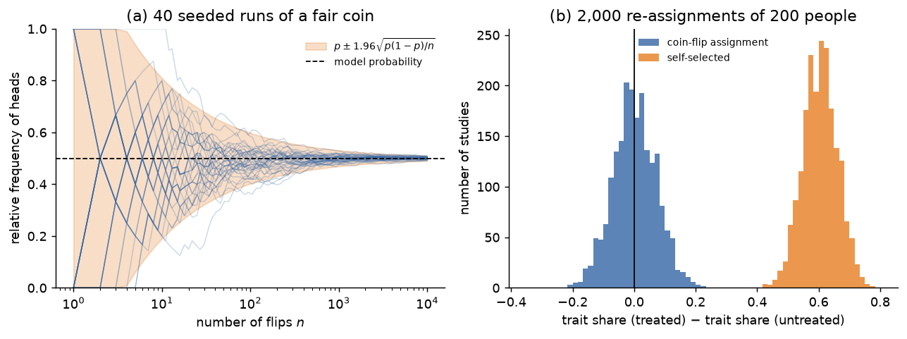

Explain. Coin-flip assignment centers the imbalance at zero. But a single small study can still be unlucky. The printed share of studies with a gap above 0.10 is not zero. That is why reports give group sizes and uncertainty. Self-selection shifts the whole distribution away from zero. More data cannot fix that.

Going deeper¶

Law of large numbers¶

Take independent trials $X_i\sim\mathrm{Bernoulli}(p)$ with $\hat p_n=\frac1n\sum_{i=1}^n X_i$ . Then

\mathbb E[\hat p_n]=p,\qquad \operatorname{Var}(\hat p_n)=\frac{p(1-p)}{n},\qquad P\big(|\hat p_n-p|\ge\varepsilon\big)\le\frac{p(1-p)}{n\varepsilon^2}\ (\text{Chebyshev}).

(2)

The central limit theorem gives the approximate pointwise band $p\pm1.96\sqrt{p(1-p)/n}$ for a fixed $n$ . A band that holds for the whole path at once must be wider. Such a band can come, for example, from the law of the iterated logarithm or from a union bound.

Randomization¶

Write $Y^t$ for the potential outcome under treatment $t$ . In the model of Section 3,

\mathbb E[Y\mid T=1]-\mathbb E[Y\mid T=0] =\underbrace{0.1}_{\text{effect}}+0.4\,\big(P(U=1\mid T=1)-P(U=1\mid T=0)\big).

(3)

Random assignment makes $T$ independent of $U$ (and so of $(Y^0,Y^1)$ ). This is called exchangeability. The second term then vanishes in expectation Hernan & Robins, 2020. Let the self-selection strength be $s$ . Then $P(U=1\mid T=1)-P(U=1\mid T=0)=2s$ when $P(U=1)=\tfrac12$ , so the bias is $0.8\,s$ .

Exercises¶

Check yourself¶

# Exercise 1
hw = 1.96 * math.sqrt((1 / 6) * (5 / 6) / 6000)
assert abs(hw - 0.0094) < 1e-4

# Exercise 2: rebuild individual flips from the running frequency, pooled over the 40 seeded runs
def flips_of(run):
    hits = np.rint(np.asarray(run["trace"]) * np.arange(1, run["n"] + 1)).astype(int)
    f = np.diff(np.concatenate([[0], hits]))
    assert set(np.unique(f)) <= {0, 1} and f.sum() == run["hits"]
    return f

after5 = []
for sd in seeds:
    f = flips_of(s.trials(0.5, 10000, seed=sd))
    w = np.convolve(f, np.ones(5, dtype=int), "valid")[:-1]      # heads among flips i-5 ... i-1
    after5.extend(f[5:][w == 5])
print(f"flips right after five heads: {len(after5)}, fraction heads: {np.mean(after5):.3f}")
assert len(after5) > 5000 and abs(np.mean(after5) - 0.5) < 0.03

# Exercise 3 and the bias formula bias = 0.8 * s
c = s.causal(prevalence=0.5, low=0.2, high=0.8, base=0.2, effect=0.1, confound=0.4)
assert math.isclose(c["observed"] - c["ate"], 0.24)
for st in strengths:
    assert math.isclose(res[st]["theory"] - TRUE_EFFECT, 0.8 * st, abs_tol=1e-12)
print("All checks passed.")

flips right after five heads: 12394, fraction heads: 0.500
All checks passed.